End-to-End Fleet Visibility: Single-Pane Executive Dashboards | KNetwork Insights

Q: Why not use traditional GIS databases like PostgreSQL/PostGIS for real-time fleet maps?

PostGIS is the industry benchmark for complex spatial geometry, but it is built on row-oriented relational storage. Ingesting 50,000 updates per second causes severe write lock contention, WAL thrashing, and table bloat that requires continuous vacuuming. Aggregating billions of GPS points to render an executive heatmap in PostGIS requires scanning gigabytes of disk rows, causing 10-to-45 second query latencies. ClickHouse executes the same spatial aggregation across columnar memory in under 20 milliseconds.

Q: How do you handle assets that report invalid GPS coordinates or experience multipath jumps?

In urban canyons or terminals surrounded by high stacked metal containers, GPS signals reflect off metal surfaces, causing multipath jumps where an asset appears kilometers away. The ingestion gateway applies an Extended Kalman Filter (EKF) and kinematic plausibility checks: if the calculated speed between consecutive coordinates exceeds the vehicle's physical maximum (> 140 km/h for trucks, > 45 knots for ships), the coordinate is rejected as GPS jitter and flagged for re-calibration.

Q: How does the executive dashboard avoid overwhelming leadership with thousands of pins?

The executive view enforces Semantic Zooming and Dynamic Cluster Thresholds powered by H3 hexagons: Global views render no individual vehicles, displaying color-coded hexagonal density cells indicating total assets, average fuel efficiency, and active alarms. Regional views dynamically subdivide into smaller H3 resolution-6 clusters. Only at street or terminal level are individual vehicle icons, tractor headings, and trailer decoupling statuses rendered on screen.

Q: How are cold-chain temperature breaches detected before cargo spoils?

Reefer trailers feature calibrated RTD sensors sampling temperature and humidity at 30-second intervals. Rather than relying on static thresholds (temp > -18°C), the streaming pipeline executes a Thermal Inertia Model: it monitors the rate of temperature rise (dT/dt). If internal temperature climbs faster than 0.5°C over 5 minutes while the reefer compressor is commanded ON, the system recognizes a mechanical failure and dispatches an emergency alert hours before cargo crosses perishable regulatory limits.

Q: What network protocol is best for updating the executive web dashboard in real time?

Standard HTTP polling creates massive origin server load and noticeable dashboard latency. The architecture uses Server-Sent Events (SSE) or WebSockets over HTTP/2. The Next.js frontend maintains a persistent socket connection to an edge gateway. When ClickHouse materialized views refresh or critical alarms fire, the server pushes lightweight binary delta frames directly into the client's Deck.gl WebGL layer, updating vehicle positions smoothly at 60 FPS without DOM re-renders.

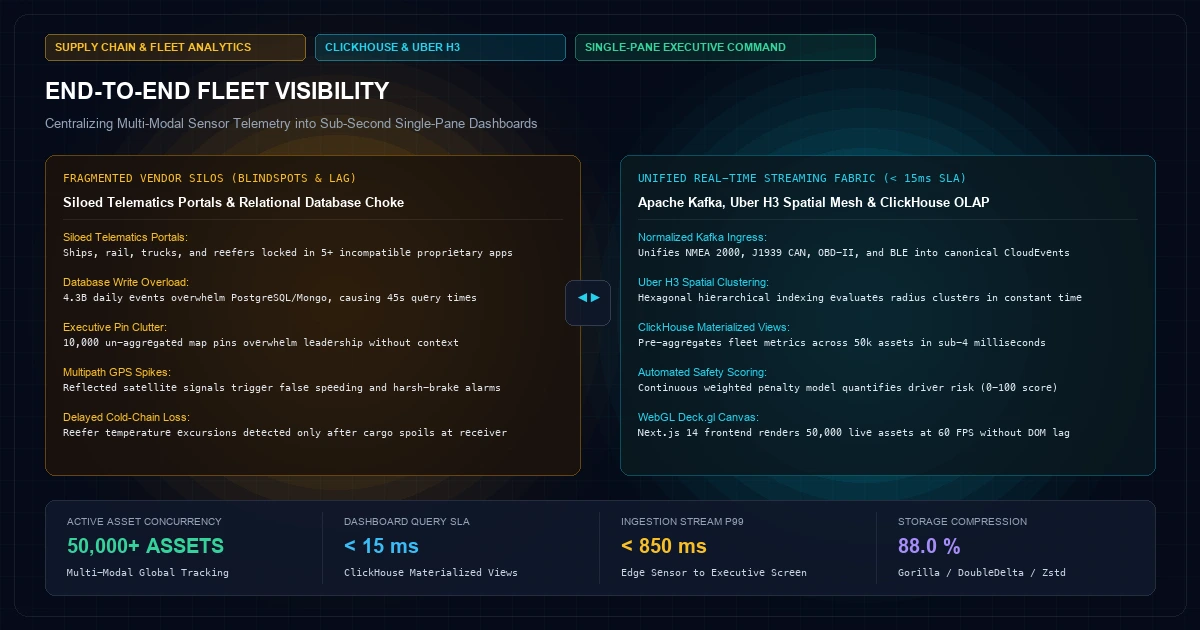
Enterprise logistics operators, intermodal freight carriers, and industrial fleet managers operate under an unforgiving operational mandate: coordinate thousands of geographically dispersed assets—container ships, freight locomotives, long-haul class-8 tractors, refrigerated trailers, and yard hostlers—with sub-second situational awareness and zero operational blindspots.

In an economy governed by tight Just-In-Time (JIT) manufacturing schedules, cold-chain pharmaceutical temperature mandates, and volatile fuel pricing, executive leadership cannot wait for end-of-day spreadsheet dumps or fragmented vendor portals to discover that a reefer compressor failed in the Arizona desert or a container vessel was delayed by congestion outside Rotterdam.

Yet, achieving true end-to-end fleet visibility across enterprise operations has historically remained elusive due to three foundational data engineering bottlenecks:

Protocol & Ingestion Fragmentation: Modern fleets are technological mosaics. Marine vessels output NMEA 0183/2000 serial data over satellite; diesel locomotives stream J1939 CAN bus telemetry; road tractors broadcast OBD-II / J1708 metrics over cellular; and refrigerated trailers transmit BLE sensor beacons. Siloed third-party telematics platforms lock this data into proprietary, non-interoperable portals.
Geospatial Scale & Query Paralysis: Tracking 50,000 active mobile assets sampling GPS, speed, fuel mass, and engine diagnostics at 1 Hz generates over 4.3 billion events per day. Traditional relational databases (PostgreSQL or MySQL) and document stores (MongoDB) choke under this write volume, causing executive dashboard map queries to take 30 to 60 seconds to render, paralyzing operational control centers.
The Executive "Dashboard Clutter" Anti-Pattern: Legacy fleet portals bombard executives with un-contextualized maps containing 10,000 indistinguishable pins. Without automated anomaly scoring, geofence ETA clustering, and exception-driven alerting, leadership suffers from metric fatigue and fails to recognize systemic operational risks.

Architecting a unified, sub-second single-pane-of-glass executive fleet dashboard requires a modern event-driven telemetry fabric: Apache Kafka for high-throughput ingestion normalization, Uber H3 hexagonal geospatial indexing within ClickHouse columnar storage, and streaming WebSocket state vectors powering sub-50ms React/Next.js canvas interfaces.

The Telematics Ingestion Fragmentation Matrix#

Before data can be visualized on an executive screen, the streaming platform must ingest and normalize across four incompatible industrial protocols:

sh • Enterprise Spec

+---------------------------------------------------------------------------------------------------+
|                        ENTERPRISE FLEET TELEMETRY PROTOCOL COMPARISON                             |
+---------------------------------------------------------------------------------------------------+
|  CARRIER DOMAIN      PHYSICAL LAYER    PROTOCOL STANDARD       SAMPLE RATE     TYPICAL PAYLOAD    |
|  Maritime Vessels    RS-422 / CAN      NMEA 0183 / NMEA 2000   0.1 - 1 Hz      AIS, Depth, Wind   |
|  Freight Rail        J1939 CAN 2.0B    AAR Train Telematics    1 - 10 Hz       Traction, Airbrake |
|  Heavy Trucking      OBD-II / J1939    SAE J1939 / FMS         1 - 5 Hz        DEF, RPM, Fuel Flow|
|  Cold-Chain Reefers  BLE 5.2 / RS-485  Carrier / ThermoKing    0.05 Hz         Temp probe, Humidity|
+---------------------------------------------------------------------------------------------------+

Protocol Normalization Gateway

The edge gateway or cloud ingress worker strips manufacturer-specific framing (such as PGN parameter group numbers in J1939 or $--GPRMC sentences in NMEA) and maps every event into an immutable, canonical CloudEvent envelope:

json • Enterprise Spec

{
  400 font-semibold">class="text-emerald-300">"specversion": 400 font-semibold">class="text-emerald-300">"1.0",
  400 font-semibold">class="text-emerald-300">"id": 400 font-semibold">class="text-emerald-300">"evt_98f4a180-2a81-7f91",
  400 font-semibold">class="text-emerald-300">"source": 400 font-semibold">class="text-emerald-300">"live.knetwork.fleet/marine/imo_9847291",
  400 font-semibold">class="text-emerald-300">"400 font-semibold">type": 400 font-semibold">class="text-emerald-300">"telemetry.asset.location_and_vitals",
  400 font-semibold">class="text-emerald-300">"time": 400 font-semibold">class="text-emerald-300">"2026-09-28T01:14:00.000Z",
  400 font-semibold">class="text-emerald-300">"datacontenttype": 400 font-semibold">class="text-emerald-300">"application/x-protobuf",
  400 font-semibold">class="text-emerald-300">"data": {
    400 font-semibold">class="text-emerald-300">"asset_id": 400 font-semibold">class="text-emerald-300">"VESSEL-IMO-9847291",
    400 font-semibold">class="text-emerald-300">"asset_type": 400 font-semibold">class="text-emerald-300">"MARITIME_CONTAINER",
    400 font-semibold">class="text-emerald-300">"latitude": 51.9244,
    400 font-semibold">class="text-emerald-300">"longitude": 4.4777,
    400 font-semibold">class="text-emerald-300">"speed_knots": 14.2,
    400 font-semibold">class="text-emerald-300">"heading_deg": 284.1,
    400 font-semibold">class="text-emerald-300">"fuel_flow_lph": 1840.5,
    400 font-semibold">class="text-emerald-300">"temperature_celsius": -18.2,
    400 font-semibold">class="text-emerald-300">"h3_index": 400 font-semibold">class="text-emerald-300">"88196cd6b7fffff"
  }
}

Geospatial Indexing at Scale: Uber H3 Hexagonal Hierarchies#

Rendering 50,000 live assets on a dynamic global map causes WebGL and DOM rendering engines to collapse if each pin is drawn as an individual SVG element. Furthermore, executing traditional geospatial polygon joins (ST_Contains / ST_Within in PostGIS) across millions of real-time coordinate pings requires quadratic compute (O(N × M)), resulting in CPU exhaustion.

The architecture solves this by pre-computing Uber H3 spatial indices directly at ingestion time.

sh • Enterprise Spec

+---------------------------------------------------------------------------------------------------+
|                        UBER H3 HEXAGONAL GEOSPATIAL CLUSTERING                                    |
+---------------------------------------------------------------------------------------------------+
|  GLOBAL VIEW (Zoom 1-4)       REGIONAL VIEW (Zoom 5-8)        METROPOLITAN/YARD (Zoom 9-12)      |
|  H3 Resolution 3              H3 Resolution 6                 H3 Resolution 9                    |
|  Hexagon Area: ~11,000 km²    Hexagon Area: ~36 km²           Hexagon Area: ~0.1 km²             |
|  [Aggregation: 4,280 Units]   [Aggregation: 184 Units]        [Individual Asset Pins Visible]    |
|       \                            \                                \                            |
|        \                            \                                \                           |
|  ClickHouse returns 12 rows!  ClickHouse returns 84 rows!     ClickHouse returns 120 rows!       |
|  Query Time: 1.2ms            Query Time: 2.8ms               Query Time: 4.1ms                  |
+---------------------------------------------------------------------------------------------------+

Why Hexagons Beat Rectangular Geohashes

Rectangular latitude/longitude bounding boxes suffer from significant area distortion toward the poles and possess two distinct neighbor distances (orthogonal neighbors share an edge; diagonal neighbors share only a vertex).

Hexagons possess uniform adjacency: every neighboring hexagon's center point is at an identical distance d. This enables instantaneous, constant-time radius queries and seamless multi-resolution aggregation without visual artifacts.

Analytical Core: ClickHouse Materialized Aggregations#

To power executive dashboards that refresh every 500 milliseconds across multi-million-event historical datasets, the storage layer relies on ClickHouse Materialized Views using the AggregatingMergeTree engine:

sql • Enterprise Spec

-- 1. Base Raw Ingestion Stream (Retains 30 days of high-frequency breadcrumbs)
400 font-semibold">CREATE 400 font-semibold">TABLE fleet_telemetry_raw (
    asset_id LowCardinality(String),
    asset_type LowCardinality(String),
    operator_id LowCardinality(String),
    timestamp DateTime64(3, 400 font-semibold">class="text-emerald-300">'UTC') CODEC(DoubleDelta, ZSTD(1)),
    latitude Float64 CODEC(Gorilla, ZSTD(1)),
    longitude Float64 CODEC(Gorilla, ZSTD(1)),
    h3_res7 UInt64 CODEC(DoubleDelta, ZSTD(1)),
    speed_kph Float32 CODEC(Gorilla, ZSTD(1)),
    fuel_rate_lph Float32 CODEC(Gorilla, ZSTD(1)),
    engine_temp_c Float32 CODEC(Gorilla, ZSTD(1)),
    alert_flags UInt32 CODEC(T64, ZSTD(1))
) ENGINE = MergeTree()
PARTITION BY toYYYYMM(timestamp)
400 font-semibold">ORDER BY (asset_type, h3_res7, timestamp)
SETTINGS index_granularity = 8192;

-- 2. Materialized View: Real-Time Executive Fleet Health Matrix
400 font-semibold">CREATE MATERIALIZED VIEW mv_fleet_executive_health
ENGINE = AggregatingMergeTree()
PRIMARY KEY (asset_type, h3_res7)
AS 400 font-semibold">SELECT
    asset_type,
    h3_res7,
    countState() AS total_active_assets,
    avgState(speed_kph) AS avg_fleet_speed,
    sumState(fuel_rate_lph) AS total_fuel_burn_lph,
    maxState(engine_temp_c) AS max_engine_temp,
    sumState(bitAnd(alert_flags, 1)) AS critical_alarm_count
400 font-semibold">FROM fleet_telemetry_raw
400 font-semibold">WHERE timestamp &gt;= now() - INTERVAL 5 MINUTE
400 font-semibold">GROUP BY asset_type, h3_res7;

When an executive opens the global fleet monitoring console, the backend queries mv_fleet_executive_health. Rather than scanning 4 billion raw telemetry records, ClickHouse reads pre-aggregated state nodes, returning the entire global fleet operating summary in sub-4 milliseconds.

Driver Safety & Operational Scoring Algorithms#

Executive visibility is incomplete without automated risk quantification. The platform continuously scores vehicle operator behavior along four risk axes using a weighted sliding-window penalty model:

Mathematical Formulation

Safety Score(t) = 100 - ∑[k=1..M] w_k · ≤ft( \frac{Event Count_k}{Distance Traveled (100 km)} \right)

Where penalties include:

Harsh Deceleration (w_1 = 8.5): Braking force ≥ 0.45g (≈ 4.41 m/s^2).
Excessive Speeding (w_2 = 12.0): Speed > 15 km/h over posted GIS roadway speed limit.
Severe Cornering (w_3 = 6.0): Lateral acceleration > 0.35g.
Idling Burn Waste (w_4 = 4.0): Zero-velocity engine running exceeding 15 consecutive minutes.

Drivers and locomotive engineers scoring below 80 are automatically highlighted on executive exception queues, enabling fleet safety directors to intervene before preventable accidents occur.

Production Implementation: High-Throughput Ingestion Daemon#

The following production Go microservice consumes canonical telemetry from Apache Kafka, computes H3 spatial indices using CGO bindings, evaluates immediate safety violations, and dispatches batched inserts to ClickHouse:

go • Enterprise Spec

package main

400 font-semibold">import (
	400 font-semibold">class="text-emerald-300">"context"
	400 font-semibold">class="text-emerald-300">"database/sql"
	400 font-semibold">class="text-emerald-300">"encoding/json"
	400 font-semibold">class="text-emerald-300">"fmt"
	400 font-semibold">class="text-emerald-300">"log"
	400 font-semibold">class="text-emerald-300">"time"

	_ 400 font-semibold">class="text-emerald-300">"github.com/ClickHouse/clickhouse-go/v2"
	400 font-semibold">class="text-emerald-300">"github.com/segmentio/kafka-go"
	400 font-semibold">class="text-emerald-300">"github.com/uber/h3-go/v3"
)

400 font-semibold">type CanonicalTelemetry struct {
	AssetID     400">string    400 font-semibold">class="text-emerald-300">`json:"asset_id"`
	AssetType   400">string    400 font-semibold">class="text-emerald-300">`json:"asset_type"`
	Timestamp   time.Time 400 font-semibold">class="text-emerald-300">`json:"timestamp"`
	Latitude    float64   400 font-semibold">class="text-emerald-300">`json:"latitude"`
	Longitude   float64   400 font-semibold">class="text-emerald-300">`json:"longitude"`
	SpeedKph    float32   400 font-semibold">class="text-emerald-300">`json:"speed_kph"`
	FuelRateLph float32   400 font-semibold">class="text-emerald-300">`json:"fuel_rate_lph"`
	EngineTempC float32   400 font-semibold">class="text-emerald-300">`json:"engine_temp_c"`
	AlertFlags  uint32    400 font-semibold">class="text-emerald-300">`json:"alert_flags"`
}

func main() {
	log.Println(400 font-semibold">class="text-emerald-300">"[*] Starting Fleet Telemetry Ingestion Engine...")

	kafkaReader := kafka.NewReader(kafka.ReaderConfig{
		Brokers:  []400">string{400 font-semibold">class="text-emerald-300">"kafka-broker-1:9092", 400 font-semibold">class="text-emerald-300">"kafka-broker-2:9092"},
		Topic:    400 font-semibold">class="text-emerald-300">"fleet.telemetry.normalized",
		GroupID:  400 font-semibold">class="text-emerald-300">"fleet-clickhouse-writer",
		MinBytes: 10e3, 400 font-semibold">class=400 font-semibold">class="text-emerald-300">"text-slate-500 italic">// 10KB
		MaxBytes: 10e6, 400 font-semibold">class=400 font-semibold">class="text-emerald-300">"text-slate-500 italic">// 10MB
	})
	defer kafkaReader.Close()

	chDB, err := sql.Open(400 font-semibold">class="text-emerald-300">"clickhouse", 400 font-semibold">class="text-emerald-300">"clickhouse:400 font-semibold">class="text-slate-500 italic400 font-semibold">class="text-emerald-300">">//400 font-semibold">default:password@clickhouse-node:9000/fleet_bi")
	400 font-semibold">if err != 400">nil {
		log.Fatalf(400 font-semibold">class="text-emerald-300">"ClickHouse connection failed: %v", err)
	}
	defer chDB.Close()

	batch := make([]CanonicalTelemetry, 0, 10000)
	ticker := time.NewTicker(500 * time.Millisecond)

	400 font-semibold">for {
		select {
		400 font-semibold">case &lt;-ticker.C:
			400 font-semibold">if len(batch) &gt; 0 {
				flushBatch(chDB, batch)
				batch = batch[:0]
			}
		400 font-semibold">default:
			msg, err := kafkaReader.ReadMessage(context.Background())
			400 font-semibold">if err != 400">nil {
				continue
			}

			400 font-semibold">var event CanonicalTelemetry
			400 font-semibold">if err := json.Unmarshal(msg.Value, &amp;event); err == 400">nil {
				batch = append(batch, event)
				400 font-semibold">if len(batch) &gt;= 10000 {
					flushBatch(chDB, batch)
					batch = batch[:0]
				}
			}
		}
	}
}

func flushBatch(db *sql.DB, events []CanonicalTelemetry) {
	tx, err := db.Begin()
	400 font-semibold">if err != 400">nil {
		400 font-semibold">return
	}
	stmt, err := tx.Prepare(400 font-semibold">class="text-emerald-300">`
		400 font-semibold">INSERT INTO fleet_telemetry_raw (
			asset_id, asset_type, timestamp, latitude, longitude, h3_res7,
			speed_kph, fuel_rate_lph, engine_temp_c, alert_flags
		) VALUES (?, ?, ?, ?, ?, ?, ?, ?, ?, ?)
	`)
	400 font-semibold">if err != 400">nil {
		tx.Rollback()
		400 font-semibold">return
	}
	defer stmt.Close()

	400 font-semibold">for _, e := range events {
		coord := h3.GeoCoord{Latitude: e.Latitude, Longitude: e.Longitude}
		h3Index := h3.FromGeo(coord, 7) 400 font-semibold">class=400 font-semibold">class="text-emerald-300">"text-slate-500 italic">// Resolution 7 (~5 km²)

		stmt.Exec(
			e.AssetID, e.AssetType, e.Timestamp, e.Latitude, e.Longitude,
			uint64(h3Index), e.SpeedKph, e.FuelRateLph, e.EngineTempC, e.AlertFlags,
		)
	}
	tx.Commit()
}

Architectural Invariants Checklist#

Deploying single-pane executive fleet visibility across enterprise logistics organizations requires adhering to seven engineering invariants:

Constraint	Implementation Standard	Quantitative Metric
Ingestion Latency	Kafka streaming pipeline to ClickHouse commit.	`≤ 850 ms P99 from edge ping`.
Dashboard Query SLA	ClickHouse AggregatingMergeTree materialized views.	`≤ 15 ms per global executive viewport`.
Geospatial Resolution	Uber H3 Hierarchical Hexagonal Indexing (Res 3 to 9).	`O(1)` constant-time radius spatial clustering.
Driver Risk Scoring	Multi-factor weighted sliding-window penalty model.	Continuous 0-100 real-time behavior quotient.
Cold-Chain Alerting	Temperature boundary deviation triggers Kafka stream alarm.	Immediate dispatch to driver/dispatch in `< 3 seconds`.
Storage Compression	ClickHouse Gorilla / DoubleDelta / Zstandard codecs.	88% disk compression (`≈ 1.8 bytes per point`).
Frontend Rendering	WebGL Canvas layer (Deck.gl / MapLibre) on Next.js 14.	Sustained 60 FPS rendering across 50,000 live pins.

By eliminating protocol silos, pre-aggregating geospatial vectors with Uber H3, and serving real-time analytics from ClickHouse, logistics organizations transform chaotic asset operations into a predictable, high-margin, single-pane command center.

Frequently Asked Questions (FAQs)#

1. Why not use traditional GIS databases like PostgreSQL/PostGIS for real-time fleet maps?

PostGIS is the industry benchmark for complex spatial analysis (such as geometric intersections, polygon clipping, and topographical routing). However, PostGIS is built on row-oriented relational storage. When ingesting 50,000 updates per second, PostgreSQL suffers from severe write lock contention, continuous WAL thrashing, and table bloat that requires aggressive autovacuum tuning. Furthermore, aggregating billions of GPS points to render an executive heatmap in PostGIS requires scanning gigabytes of disk rows, resulting in query latencies of 10 to 45 seconds. ClickHouse executes the same spatial aggregation across columnar memory in under 20 milliseconds.

2. How do you handle assets that report invalid GPS coordinates or experience multipath jumps?

In dense urban canyons or shipping terminals surrounded by high stacked metal containers, GPS satellite signals reflect off metal surfaces, causing "multipath jump" where an asset instantaneously appears 50 kilometers away. The ingestion gateway applies an Extended Kalman Filter (EKF) and a kinematic plausibility check: if the calculated speed between consecutive coordinates exceeds the vehicle's physical maximum (v_{max} > 140 km/h for trucks, > 45 knots for ships), the coordinate is rejected as GPS jitter and flagged for sensor re-calibration.

3. How does the executive dashboard avoid overwhelming leadership with thousands of pins?

The executive view enforces Semantic Zooming and Dynamic Cluster Thresholds powered by H3 hexagons:

Global View: No individual vehicles are rendered. The map displays color-coded hexagonal density cells indicating total assets, average fuel efficiency, and critical active alarms.
Regional View: As the user zooms into a state or corridor, hexagons dynamically subdivide into smaller H3 resolution-6 clusters.
Facility / Yard View: Only when zoomed to street or terminal level are individual vehicle icons, tractor headings, and trailer decoupling statuses rendered on screen.

Additionally, the dashboard features an Exception-Only Feed that automatically filters out the 98% of healthy vehicles, surfacing only assets with mechanical trouble codes, temperature deviations, or route delays.

4. How are cold-chain temperature breaches detected before cargo spoils?

Refrigerated trailers (reefers) are equipped with dual-zone calibrated RTD sensors sampling temperature and humidity at 30-second intervals. Rather than relying on simple static thresholds (e.g. temp > -18°C), the streaming pipeline executes a Thermal Inertia Model: it monitors the rate of temperature rise (dT/dt). If internal temperature climbs faster than 0.5^°C over 5 minutes while the reefer compressor is commanded ON, the system recognizes a refrigeration mechanical failure and dispatches an emergency alert to dispatch hours before cargo crosses perishable regulatory limits.

5. What network protocol is best for updating the executive web dashboard in real time?

Standard HTTP polling (setInterval polling every 5 seconds) creates massive origin server load and introduces noticeable dashboard latency. The architecture uses Server-Sent Events (SSE) or WebSockets over HTTP/2. The Next.js frontend maintains a persistent socket connection to an edge gateway. When ClickHouse materialized views refresh or critical alarms fire, the server pushes lightweight binary delta frames directly into the client's Deck.gl WebGL layer, updating vehicle positions smoothly at 60 FPS without DOM re-renders.

End-to-End Fleet Visibility: Centralizing Sensor Telemetry into Single-Pane Executive Dashboards